SWIM Example
Standard Water Integrated Model
from thermoengine import phases
from thermoengine import model
import matplotlib.pyplot as plt
import numpy as np
%matplotlib inline
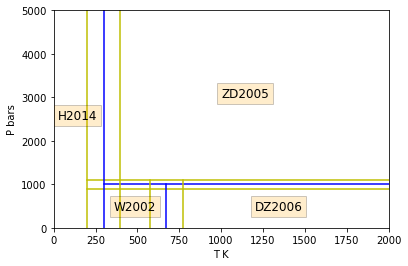
- H2014, Holten et al., 2014 - W2002, Wagner et al., 2002 - ZD2005,
Zhang and Duan, 2005 - DZ2006, Duan and Zhang, 2006
These models are merged, averaged and reconciled for all derivatives
to third order over the following regions of \(T\)-\(P\)
space.
plt.plot([198.15,2000.0],[1100.0,1100.0],'y')
plt.plot([198.15,2000.0],[ 900.0, 900.0],'y')
plt.plot([298.15,2000.0],[1000.0,1000.0],'b')
plt.plot([198.15,198.15],[0.0,5000.0],'y')
plt.plot([398.15,398.15],[0.0,5000.0],'y')
plt.plot([298.15,298.15],[0.0,5000.0],'b')
plt.plot([573.15,573.15],[0.0,1100.0],'y')
plt.plot([773.15,773.15],[0.0,1100.0],'y')
plt.plot([673.15,673.15],[0.0,1000.0],'b')
plt.ylabel('P bars')
plt.xlabel('T K')
plt.xlim(left=0.0, right=2000.0)
plt.ylim(bottom=0.0, top=5000.0)
plt.text(1000.0,3000.0,"ZD2005",fontsize=12,bbox=dict(facecolor='orange', alpha=0.2))
plt.text(1200.0, 400.0,"DZ2006",fontsize=12,bbox=dict(facecolor='orange', alpha=0.2))
plt.text( 360.0, 400.0,"W2002",fontsize=12,bbox=dict(facecolor='orange', alpha=0.2))
plt.text(  25.0,2500.0,"H2014",fontsize=12,bbox=dict(facecolor='orange', alpha=0.2))
plt.show()
Instantiate SWIM using the simple python wrappers
(Molecular weight in grams/mole)
modelDB = model.Database()
H2O = modelDB.get_phase('H2O')
print (H2O.props['phase_name'])
print (H2O.props['formula'][0])
print (H2O.props['molwt'][0])
Water
H2O
18.0152
Use the Python wrapper functions to obtain thermodynamic properties of water
\(T\) (temperature, first argument) is in K, and \(P\) (pressure, second argument) is in bars.
print ("{0:>10s}{1:15.2f}{2:<20s}".format("G", H2O.gibbs_energy(1000.0, 1000.0), 'J/mol'))
print ("{0:>10s}{1:15.2f}{2:<20s}".format("H", H2O.enthalpy(1000.0, 1000.0), 'J/mol'))
print ("{0:>10s}{1:15.2f}{2:<20s}".format("S", H2O.entropy(1000.0, 1000.0), 'J/K-mol'))
print ("{0:>10s}{1:15.3f}{2:<20s}".format("Cp", H2O.heat_capacity(1000.0, 1000.0), 'J/K-mol'))
print ("{0:>10s}{1:15.6e}{2:<20s}".format("dCp/dT", H2O.heat_capacity(1000.0, 1000.0, deriv={'dT':1}), 'J/-K^2-mol'))
print ("{0:>10s}{1:15.3f}{2:<20s}".format("V", H2O.volume(1000.0, 1000.0, deriv={'dT':1}), 'J/bar-mol'))
print ("{0:>10s}{1:15.6e}{2:<20s}".format("dV/dT", H2O.volume(1000.0, 1000.0, deriv={'dT':1}), 'J/bar-K-mol'))
print ("{0:>10s}{1:15.6e}{2:<20s}".format("dv/dP", H2O.volume(1000.0, 1000.0, deriv={'dP':1}), 'J/bar^2-mol'))
print ("{0:>10s}{1:15.6e}{2:<20s}".format("d2V/dT2", H2O.volume(1000.0, 1000.0, deriv={'dT':2}), 'J/bar-K^2-mol'))
print ("{0:>10s}{1:15.6e}{2:<20s}".format("d2V/dTdP", H2O.volume(1000.0, 1000.0, deriv={'dT':1, 'dP':1}), 'J/bar^2-K-mol'))
print ("{0:>10s}{1:15.6e}{2:<20s}".format("d2V/dP2", H2O.volume(1000.0, 1000.0, deriv={'dP':2}), 'J/bar^3-mol'))
       G     -323482.97J/mol
       H     -225835.42J/mol
       S         167.15J/K-mol
      Cp         72.914J/K-mol
  dCp/dT  -1.242746e-01J/-K^2-mol
       V          0.014J/bar-mol
   dV/dT   1.431826e-02J/bar-K-mol
   dv/dP  -7.243395e-03J/bar^2-mol
 d2V/dT2  -1.818046e-05J/bar-K^2-mol
d2V/dTdP  -1.299463e-05J/bar^2-K-mol
 d2V/dP2   1.744388e-05J/bar^3-mol
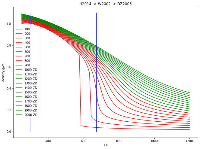
Plot the density of water as a function of \(T\) …
… for 20 isobars at 100 to 2000 bars
P_array = np.linspace(100.0, 2000.0, 20, endpoint=True) # 100->2000, 10 bars
T_array = np.linspace(250.0, 1200.0, 100, endpoint=True) # 250->1200,100 K
MW = H2O.props['molwt']
for P in P_array:
    Den_array = MW/H2O.volume(T_array, P)/10.0 ## cc
    if P < 1000.0:
        plt.plot(T_array, Den_array, 'r-', label=str(int(P)))
    else:
        plt.plot(T_array, Den_array, 'g-', label=str(int(P))+"-ZD")
plt.plot([673.15,673.15],[0.0,1.1],'b')
plt.plot([298.15,298.15],[0.0,1.1],'b')
plt.ylabel('density g/cc')
plt.xlabel('T K')
plt.title("H2014 -> W2002 -> DZ2006")
plt.legend()
fig = plt.gcf()
fig.set_size_inches(11,8)
plt.show()
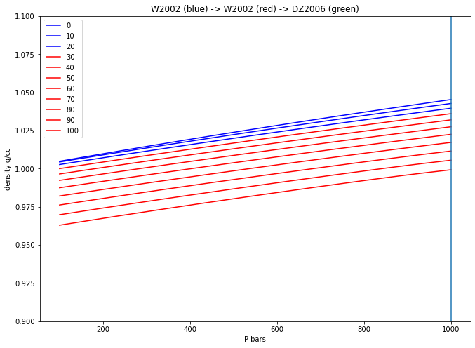
Plot the density of water as a function of \(P\) …
… for 11 isotherms at 0 to 100 °C
T_array = np.linspace(0.0, 100.0, 11, endpoint=True) # 0->100, 11 °C
P_array = np.linspace(100.0, 1000.0, 100, endpoint=True) # 100->1000, 100 bars
MW = H2O.props['molwt']
for T in T_array:
    Den_array = MW/H2O.volume(T+273.15, P_array)/10.0 ## cc
    if T <= 25.0:
        plt.plot(P_array, Den_array, 'b-', label=str(int(T)))
    elif T <= 400.0:
        plt.plot(P_array, Den_array, 'r-', label=str(int(T)))
    else:
        plt.plot(P_array, Den_array, 'g-', label=str(int(T)))
plt.plot([1000.0,1000.0],[0.9,1.3])
plt.ylabel('density g/cc')
plt.xlabel('P bars')
plt.ylim(bottom=0.9, top=1.1)
plt.title("W2002 (blue) -> W2002 (red) -> DZ2006 (green)")
plt.legend()
fig = plt.gcf()
fig.set_size_inches(11,8)
plt.show()
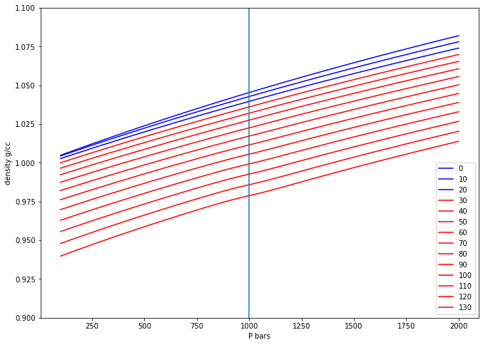
Use direct calls to Objective-C functions (via Rubicon) to select specific water models
from ctypes import cdll
from ctypes import util
from rubicon.objc import ObjCClass, objc_method
cdll.LoadLibrary(util.find_library('phaseobjc'))
Water = ObjCClass('GenericH2O')
water = Water.alloc().init()
#water.forceModeChoiceTo_("MELTS H2O-CO2 from Duan and Zhang (2006)")
#water.forceModeChoiceTo_("DEW H2O from Zhang and Duan (2005)")
#water.forceModeChoiceTo_("Supercooled H2O from Holten et al. (2014)")
#water.forceModeChoiceTo_("Steam Properties from Wagner et al. (2002)")
water.forceModeChoiceAutomatic()
T_array = np.linspace(0.0, 130.0, 14, endpoint=True)
P_array = np.linspace(100.0, 2000.0, 100, endpoint=True) # bars
MW = H2O.props['molwt']
for T in T_array:
    Den_array = np.empty_like(P_array)
    i = 0
    for P in P_array:
        Den_array[i] = MW/water.getVolumeFromT_andP_(T+273.15, P)/10.0 ## cc
        i = i + 1
    if T <= 25.0:
        plt.plot(P_array, Den_array, 'b-', label=str(int(T)))
    elif T <= 400.0:
        plt.plot(P_array, Den_array, 'r-', label=str(int(T)))
    else:
        plt.plot(P_array, Den_array, 'g-', label=str(int(T)))
fig = plt.gcf()
fig.set_size_inches(11,8)
plt.plot([1000.0,1000.0],[0.5,1.3])
plt.ylabel('density g/cc')
plt.xlabel('P bars')
plt.ylim(bottom=0.9, top=1.1)
plt.legend()
plt.show()
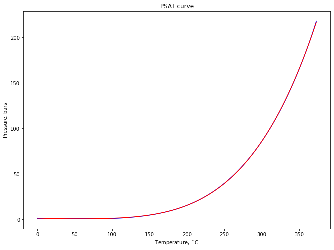
Calculations on the steam saturation curve
import pandas as pd
def vol(T=25, P=1):
    return H2O.volume(T+273.15, P)*10
psat_df = pd.read_csv('psat.csv')
from scipy.optimize import curve_fit
def func(x, a, b, c, d, e):
    return a + b*x + c*x*x + d*x*x*x + e*x*x*x*x
popt, pcov = curve_fit(func, psat_df['T'], psat_df['P'])
popt
array([ 1.44021565e+00, -2.75944904e-02,  3.50602876e-04, -2.44834016e-06,
        1.57085668e-08])
fig = plt.gcf()
fig.set_size_inches(11,8)
plt.title('PSAT curve')
plt.plot(psat_df[['T']], psat_df[['P']], "b-")
plt.plot(psat_df[['T']], func(psat_df['T'], *popt), "r-")
plt.ylabel('Pressure, bars')
plt.xlabel('Temperature, $^\\circ$C')
plt.show()
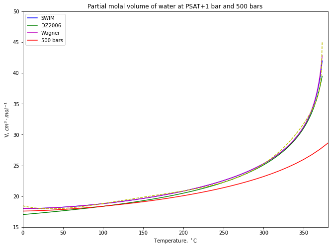
# create Psat line
volume_psat = vol(psat_df[['T']], psat_df[['P']]+1) # increase psat pressure by 1 bar to ensure liquid H2O
plt.plot(psat_df[['T']], volume_psat, "b-", label="SWIM")
Vol_array = np.empty_like(psat_df['T'])

i = 0
water.forceModeChoiceTo_("MELTS H2O-CO2 from Duan and Zhang (2006)")
for t,p in zip(psat_df['T'], psat_df['P']):
    Vol_array[i] = water.getVolumeFromT_andP_(t+273.15, p+1.0)*10.0
    i = i + 1
plt.plot(psat_df[['T']], Vol_array, "g-", label="DZ2006")

i = 0
water.forceModeChoiceTo_("Steam Properties from Wagner et al. (2002)")
for t,p in zip(psat_df['T'], psat_df['P']):
    Vol_array[i] = water.getVolumeFromT_andP_(t+273.15, p+1.0)*10.0
    i = i + 1
plt.plot(psat_df[['T']], Vol_array, "m-", label="Wagner")

def func(x, a, b, c, d, e, f):
    return a + b*x + c*x*x + d*x*x*x + e*x*x*x*x + f/(x-374.0)
popt, pcov = curve_fit(func, psat_df['T'], Vol_array)
print (popt)
plt.plot(psat_df[['T']], func(psat_df['T'], *popt), "y--")

water.forceModeChoiceAutomatic()

# create 500 bar line
temps = np.arange(0, 1010, 10)
plt.plot(temps, vol(T=temps, P=500), "r-", label="500 bars")

# plot options
fig = plt.gcf()
fig.set_size_inches(11,8)
plt.title('Partial molal volume of water at PSAT+1 bar and 500 bars')
plt.ylabel('V, $cm^{3}\\cdot mol^{-1}$')
plt.xlabel('Temperature, $^\\circ$C')
plt.margins(x=0) # no margins on x axis
plt.ylim([15, 50])
plt.xlim([0, 380])
plt.xticks(np.arange(0, 380, step=50))
plt.legend()
plt.show()
[ 1.84252342e+01 -3.06586710e-02  5.65750627e-04 -2.69937313e-06
  4.67555414e-09 -8.89632469e+00]