MELTS
Versions of MELTS implemented are:
- MELTS v. 1.0.2 ➞ (rhyolite-MELTS, Gualda et al., 2012)
- MELTS v. 1.1.0 ➞ (rhyolite-MELTS + new CO2, works at the ternary
minimum)
- MELTS v. 1.2.0 ➞ (rhyolite-MELTS + new H2O + new CO2)
- pMELTS v. 5.6.1
Initialize tools and packages that are required to execute this notebook.
from thermoengine import equilibrate
import matplotlib.pyplot as plt
import numpy as np
%matplotlib inline
Create a MELTS v 1.0.2 instance.
Rhyolite-MELTS version 1.0.2 is the default model.
melts = equilibrate.MELTSmodel()
Optional: Generate some information about the implemented model.
oxides = melts.get_oxide_names()
phases = melts.get_phase_names()
#print (oxides)
#print (phases)
Required: Input initial composition of the system (liquid), in wt% or grams of oxides.
Mid-Atlantic ridge MORB composition
feasible = melts.set_bulk_composition({'SiO2':  48.68,
                                       'TiO2':   1.01,
                                       'Al2O3': 17.64,
                                       'Fe2O3':  0.89,
                                       'Cr2O3':  0.0425,
                                       'FeO':    7.59,
                                       'MnO':    0.0,
                                       'MgO':    9.10,
                                       'NiO':    0.0,
                                       'CoO':    0.0,
                                       'CaO':   12.45,
                                       'Na2O':   2.65,
                                       'K2O':    0.03,
                                       'P2O5':   0.08,
                                       'H2O':    0.2})
Optional: Suppress phases that are not required in the simulation.
b = melts.get_phase_inclusion_status()
melts.set_phase_inclusion_status({'Nepheline':False, 'OrthoOxide':False})
a = melts.get_phase_inclusion_status()
for phase in b.keys():
    if b[phase] != a[phase]:
        print ("{0:<15s} Before: {1:<5s} After: {2:<5s}".format(phase, repr(b[phase]), repr(a[phase])))
Nepheline       Before: True  After: False
OrthoOxide      Before: True  After: False
Compute the equilibrium state at some specified T (°C) and P (MPa).
Print status of the calculation.
output = melts.equilibrate_tp(1220.0, 100.0, initialize=True)
(status, t, p, xmlout) = output[0]
print (status, t, p)
success, Minimal energy computed. 1220.0 100.0
Summary output of equilibrium state …
melts.output_summary(xmlout)
dict = melts.get_dictionary_of_affinities(xmlout, sort=True)
for phase in dict:
    (affinity, formulae) = dict[phase]
    if affinity < 10000.0:
        print ("{0:<20s} {1:10.2f} {2:<60s}".format(phase, affinity, formulae))
T (°C)      1220.00
P (MPa)      100.00
Plagioclase       1.4715 (g)  K0.00Na0.19Ca0.81Al1.81Si2.19O8
Spinel            0.0215 (g)  Fe''0.23Mg0.79Fe'''0.20Al1.32Cr0.45Ti0.02O4
Liquid           98.8695 (g)  wt %:SiO2 48.53 TiO2  1.02 Al2O3 17.33 Fe2O3  0.90 Cr2O3  0.04 FeO  7.67 MnO  0.00
                                  MgO  9.20 NiO  0.00 CoO  0.00 CaO 12.34 Na2O  2.65 K2O  0.03 P2O5  0.08 H2O
Olivine                  118.94 (Ca0.00Mg0.00Fe''0.50Mn0.50Co0.00Ni0.00)2SiO4
Augite                  1333.92 Na0.00Ca0.50Fe''0.00Mg1.50Fe'''0.00Ti0.00Al0.00Si2.00O6
Orthopyroxene           2294.69 Na0.00Ca0.50Fe''0.00Mg1.50Fe'''0.00Ti0.00Al0.00Si2.00O6
Forsterite              3494.95 Mg2SiO4
Quartz                  9073.52 SiO2
Obtain default set of fractionation coefficients (retain liquids, fractionate solids and fluids)
frac_coeff = melts.get_dictionary_of_default_fractionation_coefficients()
print (frac_coeff)
{'Actinolite': 1.0, 'Aegirine': 1.0, 'Aenigmatite': 1.0, 'Akermanite': 1.0, 'Andalusite': 1.0, 'Anthophyllite': 1.0, 'Apatite': 1.0, 'Augite': 1.0, 'Biotite': 1.0, 'Chromite': 1.0, 'Coesite': 1.0, 'Corundum': 1.0, 'Cristobalite': 1.0, 'Cummingtonite': 1.0, 'Fayalite': 1.0, 'Forsterite': 1.0, 'Garnet': 1.0, 'Gehlenite': 1.0, 'Hematite': 1.0, 'Hornblende': 1.0, 'Ilmenite': 1.0, 'Ilmenite ss': 1.0, 'Kalsilite': 1.0, 'Kalsilite ss': 1.0, 'Kyanite': 1.0, 'Leucite': 1.0, 'Lime': 1.0, 'Liquid': 0.0, 'Liquid Alloy': 1.0, 'Magnetite': 1.0, 'Melilite': 1.0, 'Muscovite': 1.0, 'Nepheline': 1.0, 'Nepheline ss': 1.0, 'Olivine': 1.0, 'OrthoOxide': 1.0, 'Orthopyroxene': 1.0, 'Panunzite': 1.0, 'Periclase': 1.0, 'Perovskite': 1.0, 'Phlogopite': 1.0, 'Pigeonite': 1.0, 'Plagioclase': 1.0, 'Quartz': 1.0, 'Rutile': 1.0, 'Sanidine': 1.0, 'Sillimanite': 1.0, 'Solid Alloy': 1.0, 'Sphene': 1.0, 'Spinel': 1.0, 'Titanaugite': 1.0, 'Tridymite': 1.0, 'Water': 1.0, 'Whitlockite': 1.0}
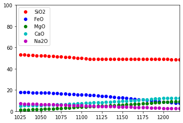
Run the sequence of calculations along a T, P=constant path:
Output is sent to an Excel file and plotted in the notebook
number_of_steps = 40
t_increment_of_steps = -5.0
p_increment_of_steps = 0.0

plotOxides = ['SiO2', 'FeO', 'MgO', 'CaO', 'Na2O']
# matplotlib colors b : blue, g : green, r : red, c : cyan, m : magenta, y : yellow, k : black, w : white.
plotColors = [ 'ro', 'bo', 'go', 'co', 'mo']

wb = melts.start_excel_workbook_with_sheet_name(sheetName="Summary")
melts.update_excel_workbook(wb, xmlout)

n = len(plotOxides)
xPlot = np.zeros(number_of_steps+1)
yPlot = np.zeros((n, number_of_steps+1))
xPlot[0] = t
for i in range (0, n):
    oxides = melts.get_composition_of_phase(xmlout, 'Liquid')
    yPlot[i][0] = oxides[plotOxides[i]]

plt.ion()
fig = plt.figure()
ax = fig.add_subplot(111)
ax.set_xlim([min(t, t+t_increment_of_steps*number_of_steps), max(t, t+t_increment_of_steps*number_of_steps)])
ax.set_ylim([0., 100.])
graphs = []
for i in range (0, n):
    graphs.append(ax.plot(xPlot, yPlot[i], plotColors[i]))
handle = []
for (graph,) in graphs:
    handle.append(graph)
ax.legend(handle, plotOxides, loc='upper left')

for i in range (1, number_of_steps):
    # fractionate phases
    frac_output = melts.fractionate_phases(xmlout, frac_coeff)
    output = melts.equilibrate_tp(t+t_increment_of_steps, p+p_increment_of_steps, initialize=True)
    (status, t, p, xmlout) = output[0]
    print ("{0:<30s} {1:8.2f} {2:8.2f}".format(status, t, p))
    xPlot[i] = t
    for j in range (0, n):
        oxides = melts.get_composition_of_phase(xmlout, 'Liquid')
        yPlot[j][i] = oxides[plotOxides[j]]
    j = 0
    for (graph,) in graphs:
        graph.set_xdata(xPlot)
        graph.set_ydata(yPlot[j])
        j = j + 1
    fig.canvas.draw()
    melts.update_excel_workbook(wb, xmlout)

melts.write_excel_workbook(wb, "MELTSv102summary.xlsx")
success, Minimal energy computed.  1215.00   100.00
success, Optimal residual norm.  1210.00   100.00
success, Minimal energy computed.  1205.00   100.00
success, Optimal residual norm.  1200.00   100.00
success, Minimal energy computed.  1195.00   100.00
success, Minimal energy computed.  1190.00   100.00
success, Optimal residual norm.  1185.00   100.00
success, Optimal residual norm.  1180.00   100.00
success, Optimal residual norm.  1175.00   100.00
success, Optimal residual norm.  1170.00   100.00
success, Optimal residual norm.  1165.00   100.00
success, Optimal residual norm.  1160.00   100.00
success, Optimal residual norm.  1155.00   100.00
success, Optimal residual norm.  1150.00   100.00
success, Optimal residual norm.  1145.00   100.00
success, Optimal residual norm.  1140.00   100.00
success, Optimal residual norm.  1135.00   100.00
success, Optimal residual norm.  1130.00   100.00
success, Optimal residual norm.  1125.00   100.00
success, Optimal residual norm.  1120.00   100.00
success, Optimal residual norm.  1115.00   100.00
success, Optimal residual norm.  1110.00   100.00
success, Optimal residual norm.  1105.00   100.00
success, Minimal energy computed.  1100.00   100.00
success, Trivial case with no quadratic search.  1095.00   100.00
success, Optimal residual norm.  1090.00   100.00
success, Optimal residual norm.  1085.00   100.00
success, Optimal residual norm.  1080.00   100.00
success, Optimal residual norm.  1075.00   100.00
success, Optimal residual norm.  1070.00   100.00
success, Optimal residual norm.  1065.00   100.00
success, Optimal residual norm.  1060.00   100.00
success, Optimal residual norm.  1055.00   100.00
success, Optimal residual norm.  1050.00   100.00
success, Optimal residual norm.  1045.00   100.00
success, Optimal residual norm.  1040.00   100.00
success, Optimal residual norm.  1035.00   100.00
success, Optimal residual norm.  1030.00   100.00
success, Optimal residual norm.  1025.00   100.00