Compare Stoichiometric Phases from Different Databases
import matplotlib.pyplot as plt
import numpy as np
%matplotlib inline
from thermoengine import phases
from thermoengine import model
modelDB = model.Database()
modelDBStix = model.Database(database='Stixrude')
modelDBHP = model.Database(database='HollandAndPowell')
Get access to a thermodynamic database (by default, the Berman (1988) database).
To print a list of all of the phases in the database, execute:
print(model.all_purephases_df.to_string())
Create the Quartz stoichiometric phase class in three databases:
Quartz_Berman = modelDB.get_phase('Qz')
Quartz_SLB = modelDBStix.get_phase('Qz')
Quartz_HP = modelDBHP.get_phase('Qz')
Perform a sanity check.
Make sure that we are not going to compare apples and oranges.
print ('{0:>10s} {1:>10s} {2:>10s}'.format('Berman DB', 'SLB DB', 'HP DB'))
print ('{0:>10s} {1:>10s} {2:>10s}'.format(
    Quartz_Berman.props['phase_name'], Quartz_SLB.props['phase_name'], Quartz_HP.props['phase_name']))
print ('{0:>10s} {1:>10s} {2:>10s}'.format(
    Quartz_Berman.props['formula'][0], Quartz_SLB.props['formula'][0], Quartz_HP.props['formula'][0]))
print ('{0:10.3f} {1:10.3f} {2:10.3f}'.format(
    Quartz_Berman.props['molwt'][0], Quartz_SLB.props['molwt'][0], Quartz_HP.props['molwt'][0]))
Berman DB     SLB DB      HP DB
   Quartz     Quartz     Quartz
     SiO2       SiO2       SiO2
   60.084     60.084     60.084
Recall that all pure component (stoichiometric) phases implement the following functions:
get_gibbs_energy(T, P)
get_enthalpy(T, P)
get_entropy(T, P)
get_heat_capacity(T, P)
get_dCp_dT(T, P)
get_volume(T, P)
get_dV_dT(T, P)
get_dV_dP(T, P)
get_d2V_dT2(T, P)
get_d2V_dTdP(T, P)
get_d2V_dP2(T, P)
where T (temperature) is in K, and P (pressure) is in bars.
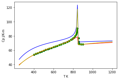
Compare the heat capacity at 1 bar.
Also, plot measured heat capacity from an especially reliable source: Ghiorso et al., 1979, Contributions to Mineralogy and Petrology v. 68, 307-323.
msg = np.loadtxt(open("Ghiorso-cp-quartz.txt", "rb"), delimiter=",", skiprows=1)
msg_data_T = msg[:,0]
msg_data_Cp = msg[:,1]

T_array = np.linspace(250.0, 1200.0, 100, endpoint=True)
Cp_array_Berman = Quartz_Berman.heat_capacity(T_array, 1.0)
Cp_array_SLB = Quartz_SLB.heat_capacity(T_array, 1.0)
Cp_array_HP = Quartz_HP.heat_capacity(T_array, 1.0)
plt.plot(msg_data_T, msg_data_Cp, 'go', T_array, Cp_array_Berman, 'r-', T_array, Cp_array_SLB, 'b-',
        T_array, Cp_array_HP, 'y-')
plt.ylabel('Cp J/K-m')
plt.xlabel('T K')
plt.show()
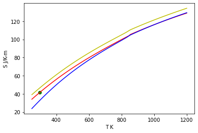
Compare the entropy at 1 bar.
Data point is reported by CODATA (1978).
S_array_Berman = Quartz_Berman.entropy(T_array, 1.0)
S_array_SLB = Quartz_SLB.entropy(T_array, 1.0)
S_array_HP = Quartz_HP.entropy(T_array, 1.0)
plt.plot(298.15, 41.46, 'go', T_array, S_array_Berman, 'r-', T_array, S_array_SLB, 'b-', T_array, S_array_HP, 'y-')
plt.ylabel('S J/K-m')
plt.xlabel('T K')
plt.show()
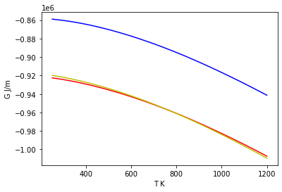
Compare the Gibbs free energy at 1 bar.
G_array_Berman = Quartz_Berman.gibbs_energy(T_array, 1.0)
G_array_SLB = Quartz_SLB.gibbs_energy(T_array, 1.0)
G_array_HP = Quartz_HP.gibbs_energy(T_array, 1.0)
plt.plot(T_array, G_array_Berman, 'r-', T_array, G_array_SLB, 'b-', T_array, G_array_HP, 'y-')
plt.ylabel('G J/m')
plt.xlabel('T K')
plt.show()
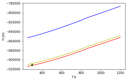
Compare the enthalpy of formation at 1 bar.
Data point is reported by CODATA (1978)
H_array_Berman = Quartz_Berman.enthalpy(T_array, 1.0)
H_array_SLB = Quartz_SLB.enthalpy(T_array, 1.0)
H_array_HP = Quartz_HP.enthalpy(T_array, 1.0)
plt.plot(298.15, -910700.0, 'go', T_array, H_array_Berman, 'r-', T_array, H_array_SLB, 'b-',
         T_array, H_array_HP, 'y-')
plt.ylabel('H J/m')
plt.xlabel('T K')
plt.show()
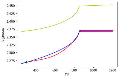
Compare the volume at 1 bar.
V_array_Berman = Quartz_Berman.volume(T_array, 1.0)
V_array_SLB = Quartz_SLB.volume(T_array, 1.0)
V_array_HP = Quartz_HP.volume(T_array, 1.0)
plt.plot(298.15, 2.269, 'go', T_array, V_array_Berman, 'r-', T_array, V_array_SLB, 'b-', T_array, V_array_HP, 'y-')
plt.ylabel('V J/bar-m')
plt.xlabel('T K')
plt.show()
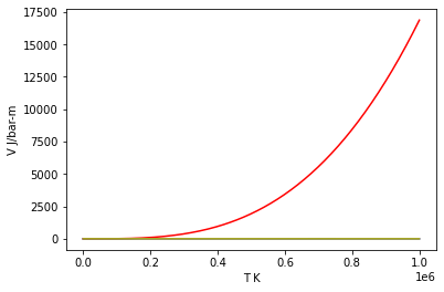
… How about the volume as a function of P?
P_array = np.linspace(1.0, 1000000.0, 200, endpoint=True)
V_array_Berman = Quartz_Berman.volume(298.15, P_array)
V_array_SLB = Quartz_SLB.volume(298.15, P_array)
V_array_HP = Quartz_HP.volume(298.15, P_array)
plt.plot(P_array, V_array_Berman, 'r-', P_array, V_array_SLB, 'b-', P_array, V_array_HP, 'y-')
plt.ylabel('V J/bar-m')
plt.xlabel('T K')
plt.show()
What does \(\frac{{\partial V}}{{\partial P}}\) look like?
dVdP_array_Berman = Quartz_Berman.volume(298.15, P_array, deriv={'dP':1})
dVdP_array_SLB = Quartz_SLB.volume(298.15, P_array, deriv={'dP':1})
dVdP_array_HP = Quartz_HP.volume(298.15, P_array, deriv={'dP':1})
plt.plot(P_array, dVdP_array_Berman, 'r-', P_array, dVdP_array_SLB, 'b-', P_array, dVdP_array_HP, 'y-')
plt.ylabel('dV/dP J/bar^2-m')
plt.xlabel('P bars')
plt.ticklabel_format(style='sci', axis='y', scilimits=(0,0))
plt.show()
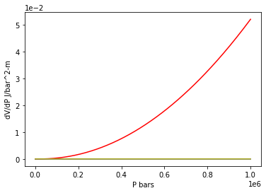
Berman (1988) using the following form: \(V = {V_0}\left[ {{v_1}\left( {P - {P_0}} \right) + {v_2}{{\left( {P - {P_0}} \right)}^2} + {v_3}\left( {T - {T_0}} \right) + {v_4}{{\left( {T - {T_0}} \right)}^2}} \right]\), whereas Stixrude and Lithgow-Bertelloni use this form: \(P = \frac{{3K}}{2}\left[ {{{\left( {\frac{{{V_0}}}{V}} \right)}^{\frac{7}{3}}} - {{\left( {\frac{{{V_0}}}{V}} \right)}^{\frac{5}{3}}}} \right]\left\{ {1 + \frac{3}{4}\left( {K' - 4} \right)\left[ {{{\left( {\frac{{{V_0}}}{V}} \right)}^{\frac{2}{3}}} - 1} \right]} \right\}\)
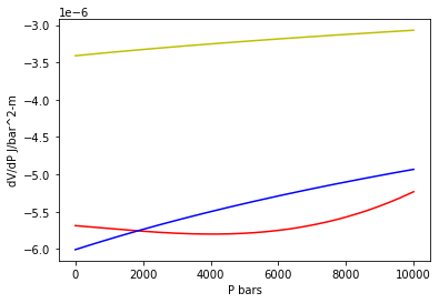
… Perhaps Berman (1988) is better at low pressure?
P_array = np.linspace(1.0, 10000.0, 200, endpoint=True)
dVdP_array_Berman = Quartz_Berman.volume(298.15, P_array, deriv={'dP':1})
dVdP_array_SLB = Quartz_SLB.volume(298.15, P_array, deriv={'dP':1})
dVdP_array_HP = Quartz_HP.volume(298.15, P_array, deriv={'dP':1})
plt.plot(P_array, dVdP_array_Berman, 'r-', P_array, dVdP_array_SLB, 'b-', P_array, dVdP_array_HP, 'y-')
plt.ylabel('dV/dP J/bar^2-m')
plt.xlabel('P bars')
plt.ticklabel_format(style='sci', axis='y', scilimits=(0,0))
plt.show()